Recently my girlfriend has been learning about autoencoders in a deep learning class she’s taking for her master’s degree and it’s caught my interest. I decided to try my hand at creating some pretty basic autoencoder architectures, utilizing the Keras architechture from Tensorflow in Python. All of the code for the project and generated figures can be found in the Fun_with_Autoencoders Jupyter Notebook located on my Github.

What is an Autoencoder?

An autoencoder is a type of neural network that is used in artificial intelligence to create efficient encodings of unlabeled data. The network hopes to learn as much as it can about the fundamental aspects of a given set of data by picking out some of the more important features or patterns that may exist. Therefore an autoencoder works to dimensionally reduce a set of data, similar to what is done in Principal Component Analysis (PCA). Among many things, these types of models excel at facial recognition, word detection, and as we shall see towards the end of this post, image reconstruction.

We can begin by importing all of the necessary packages, such as Keras for the machine learning, NumPy for data manipulation, and Matplotlib for visualizations.

''' For Machine Learning ''' 
from keras.layers import Input, Dense,Flatten
from keras.models import Model, Sequential
from keras.datasets import mnist

''' For Data Manipulation '''
import numpy as np
from sklearn.model_selection import train_test_split

''' For Visualization '''
import matplotlib.pyplot as plt

''' Other '''
import itertools
from tqdm.notebook import tnrange 

Crude Model with Uncorrelated Data

Before we can even discuss building a model, it is important to have some idea of what type of data we will be using. Now usually these types of tasks are great for feature reduction of images, and while we will get to that later, it might be a good starting point to just use some easy to control, randomly generated data, whose features are essentially uncorrelated. While this might not lead to any super interesting or meaningful results, there are still a few things we can look at such as how the number of features impacts the performance, as well as how different models stack up against each other. So, using NumPy, let’s create 1,000,000 data points with 32 features that contain random values between 0 and 1:

data = np.random.rand(1000000, 32) # Generate 1,000,000 random data points with 32 features each
train, test = train_test_split(data, test_size = 0.1, random_state = 42) # split training and testing data 

So essentially we have 1 million data points with 32 features each, and then split 90% of that data for training, and 10% for testing. Now it’s time to build our model. To start, let’s just construct the very simpliest of autoencoders that consists of 1 encoding layer and 1 decoding layer. To simplify things even further, let’s just use 2 nodes for the hidden layer. Since our data is uncorrelated to begin with, the actviation function shouldn’t matter all too much, but since our input values are all positive and between 0 and 1, let’s use the sigmoid activation:

input_dim = len(data[0]) # input dimension is equal to the number of features
hidden_layer_nodes = 2 # the number of nodes to use in the hidden layer

''' Create the Autoencoder '''
input_layer = Input(shape=(input_dim,))
encoder_layer = Dense(hidden_layer_nodes, activation='sigmoid')(input_layer)
decoder_layer = Dense(input_dim, activation='sigmoid')(encoder_layer)
autoencoder = Model(input_layer, decoder_layer)

''' Create the Encoder '''
encoder = Model(input_layer, encoder_layer)

''' Create the Decoder '''
encoded_input = Input(shape=(hidden_layer_nodes,))
decoder_layer = autoencoder.layers[-1]
decoder = Model(encoded_input, decoder_layer(encoded_input))

Great! So we take a 32 feature input, compress it down to 2 features, and then back to 32 for the output. Now we just need need to compile our model, where we will use adam for the optimizer as well as binary_crossentropy for the loss function, both of which are standard practices for building autoencoders:

autoencoder.compile(optimizer='adam', loss = 'binary_crossentropy') # compile the model

Finally let’s fit our model to our training data, and use the test data we set aside for validation. Just to keep training time light I will use a batch_size of 100 and only train for 10 epochs:

autoencoder.fit(train,
                train,
                epochs=10, # run through the training data 10 times
                batch_size=100, # use batches of 100 before making changes
                shuffle=True, # shuffle the training data to prevent biasing
                validation_data=(test, test), # use our test data set as validation
                verbose = 0) # hide the output while training

And we are done! That was easy. Now how did it do? Let’s look at the first test data point and compare it with the result after passing it through our autoencoder:

encoded_test = encoder.predict(test) # encode our features
decoded_test = decoder.predict(encoded_test) # decode our encoded features

print(test[0]) # look at the actual test value
print(decoded_test[0]) # look at the reconstructed test value

[0.556486   0.58612267 0.43598429 0.68282666 0.42345375 0.97432931
49944351 0.10358606 0.2795492  0.33025213 0.65473529 0.93899687
99052735 0.83792705 0.83594489 0.20536917 0.10406014 0.8230105
86663848 0.68582927 0.25397477 0.84576008 0.82777497 0.27917432
06123279 0.37242095 0.99979739 0.12593275 0.47674639 0.25945843
31310348 0.7138106 ]
[0.53921926 0.4994602  0.49328583 0.49671558 0.5022028  0.5054807
4923939  0.50397915 0.5014668  0.5021777  0.4975547  0.5055389
49808562 0.5042102  0.49124807 0.49604833 0.4979566  0.5032116
5059231  0.49701744 0.50652647 0.5090825  0.49114063 0.5111462
50072366 0.5080269  0.49587056 0.49579388 0.5297682  0.22143435
5013049  0.5169519 ]

Not too shabby! Some of the values are definitely in the right ballpark, but there are still a lot that aren’t even close. Generally this is okay, since we don’t always want the output to be exactly the same as the input, but it should at least be close. We can get an idea of the performance by looking at the sum of the absolute error across each feature for every data point.

\[error = \sum_{i = 1}^N|y_i - \hat{y}_i|\]

Where the sum runs over the number of features N (in our case N = 32), \(y_i\) is the \(i^{th}\) feature of the autoencoder output (the guess), and \(\hat{y}_i\) is the \(i^{th}\) feature of the actual label (the real value). If every output feature is exactly the same as the input, then we expect the error for that data point to go to zero, indicating perfect reconstruction.

error = np.sum(abs(test - decoded_test), axis = 1) # compute the absolute error across each feature 

Let’s visualize the computed errors over the entire test data set (100,000 instances) in a histogram:

fig, ax = plt.subplots(figsize = (15,8))
bins = np.linspace(min(error), max(error), 100)
ax.hist(error, bins = bins, align = 'mid', edgecolor = 'black')
ax.set_title('Simple Autoencoder Results', fontsize = 24)
ax.set_xlabel('Error', fontsize = 20)
ax.set_ylabel('Number of Counts', fontsize = 20)
ax.grid(linestyle = '--')
plt.show()

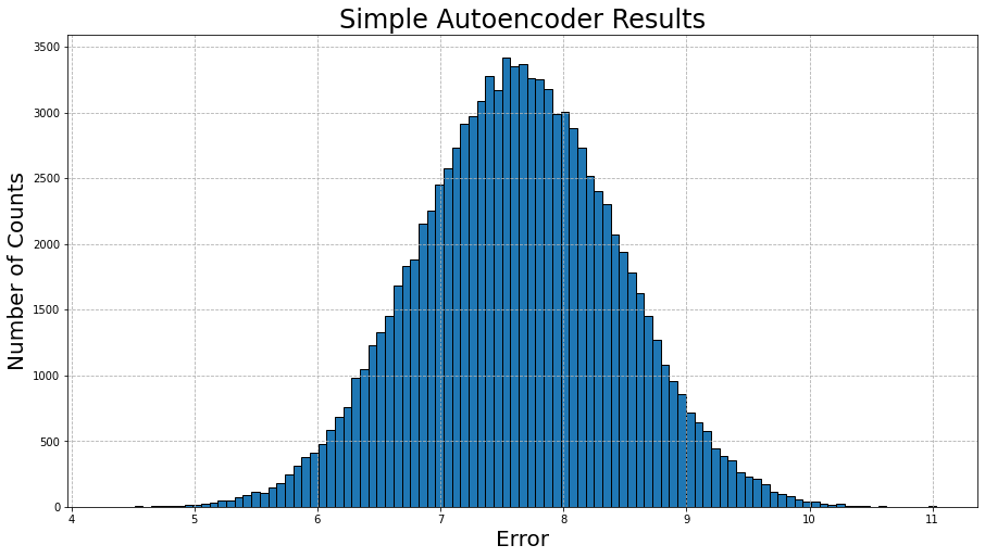
A Gaussian distribution! This actually makes a lot of sense though, as the model is trying to figure out patterns in data that ultimately has no patterns! It can only try to minimize the average error across all instances, and there will be some instances where there error is much lower or much higher.

More Complex Model with Uncorrelated Data

Now what if we tried the same thing with a more complex model? Would the results change at all? Let’s use 4 encoding layers and 4 decoding layers, with each layer decreasing/increasing by a factor of 2 (i.e. 32 -> 16 -> 8 -> 4 -> 2 -> 4 -> 8 -> 16 -> 32). We will again use sigmoid activation functions as well as the same optimizer and loss function from the simple model:

input_dim = len(data[0]) # input dimension is equal to the number of features
hidden_layer1_nodes = 16 # the number of nodes to use in the 1st hidden layer
hidden_layer2_nodes = 8 # the number of nodes to use in the 2nd hidden layer
hidden_layer3_nodes = 4 # the number of nodes to use in the 3rd hidden layer
hidden_layer4_nodes = 2 # the number of nodes to use in the 3rd hidden layer


''' Create the Autoencoder '''
input_layer = Input(shape=(input_dim,))
encoder_layer1 = Dense(hidden_layer1_nodes, activation='sigmoid')(input_layer)
encoder_layer2 = Dense(hidden_layer2_nodes, activation='sigmoid')(encoder_layer1)
encoder_layer3 = Dense(hidden_layer3_nodes, activation='sigmoid')(encoder_layer2)
encoder_layer4 = Dense(hidden_layer4_nodes, activation='sigmoid')(encoder_layer3)

decoder_layer1 = Dense(input_dim, activation='sigmoid')(encoder_layer4)
decoder_layer2 = Dense(input_dim, activation='sigmoid')(decoder_layer1)
decoder_layer3 = Dense(input_dim, activation='sigmoid')(decoder_layer2)
decoder_layer4 = Dense(input_dim, activation='sigmoid')(decoder_layer3)

autoencoder = Model(input_layer, decoder_layer4)

''' Create the Encoder '''
encoder = Model(input_layer, encoder_layer4)

''' Create the Decoder '''
encoded_input = Input(shape=(hidden_layer4_nodes,))
decoder_layer_1 = autoencoder.layers[-4]
decoder_layer_2 = autoencoder.layers[-3]
decoder_layer_3 = autoencoder.layers[-2]
decoder_layer_4 = autoencoder.layers[-1]

decoder = Model(encoded_input, decoder_layer_4(decoder_layer_3(decoder_layer_2(decoder_layer_1(encoded_input)))))

autoencoder.compile(optimizer='adam', loss = 'binary_crossentropy') # compile the model

autoencoder.fit(train,
                train,
                epochs=10, # run through the training data 10 times
                batch_size=100, # use batches of 100 before making changes
                shuffle=True, # shuffle the training data to prevent biasing
                validation_data=(test, test), # use our test data set as validation
                verbose = 0) # hide the output while training

encoded_test = encoder.predict(test) # encode our features
decoded_test = decoder.predict(encoded_test) # decode our encoded features

print(test[0]) # look at the actual test value
print(decoded_test[0]) # look at the reconstructed test value

[0.556486   0.58612267 0.43598429 0.68282666 0.42345375 0.97432931
49944351 0.10358606 0.2795492  0.33025213 0.65473529 0.93899687
99052735 0.83792705 0.83594489 0.20536917 0.10406014 0.8230105
86663848 0.68582927 0.25397477 0.84576008 0.82777497 0.27917432
06123279 0.37242095 0.99979739 0.12593275 0.47674639 0.25945843
31310348 0.7138106 ]
[0.5235458  0.5256356  0.5096446  0.79323983 0.51500344 0.5038291
48975173 0.5103137  0.5213022  0.48451337 0.5384443  0.504355
5069203  0.4980652  0.49509197 0.532431   0.5269899  0.5134901
46503198 0.5058428  0.49001136 0.49506173 0.5165646  0.49450803
4629777  0.47933778 0.46951854 0.5075482  0.5309669  0.5300103
2258296  0.5555568 ]

Again not too bad! But how does it look compared to the simple model?

fig, ax = plt.subplots(figsize = (15,8))
bins = np.linspace(min(error2), max(error2), 100)
ax.hist(error, bins = bins, align = 'mid', edgecolor = 'black', 
    label = r'1 Layer Autoencoder: $\sigma = %s$' % round(np.std(error), 3), alpha = 0.75)
ax.hist(error2, bins = bins, align = 'mid', edgecolor = 'black', 
    label = r'4 Layer Autoencoder: $\sigma = %s$' % round(np.std(error2), 3), alpha = 0.75)
ax.set_title('Comparison', fontsize = 24)
ax.set_xlabel('Error', fontsize = 20)
ax.set_ylabel('Number of Counts', fontsize = 20)
ax.grid(linestyle = '--')
ax.legend(fontsize = 18)
plt.show()

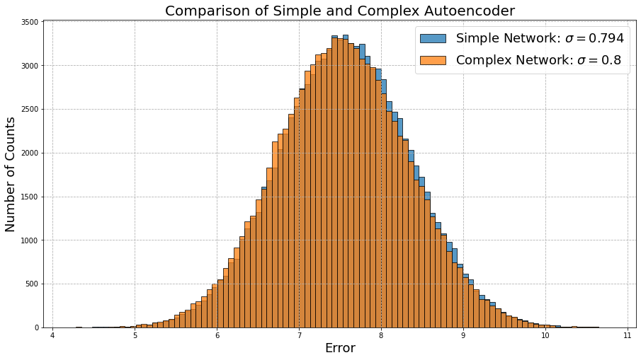
They’re almost identical! We might have naively expected the more complex model to outperform the simple model, but clearly it doesn’t matter how complex the model is if the data has no discernable patterns. Scientifically, we would say that neither model is accurate (the error is high), nor precise (there is a lot of spread). Once again, we are reminded how important the quality of data is in machine learning problems!

Do the Number of Features Matter?

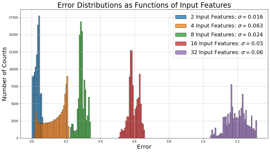
Before we move on from using data without any patterns (i.e., useless), let’s look at how important the number of features is when passed through our simple model of 1 encoding layer and 1 decoding layer from before:

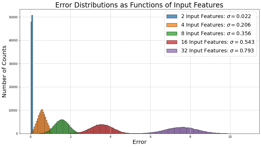
Now this is interesting! The performance of the model becomes worse as the number of features is increased. Again this makes a lot of sense! Since our generated data is uncorrelated and impossible to deduce any patterns from, the error will increase exponentially as the number of features increases.

What About More Correlated Data?

Alright now that we have had our fun with some useless data, what happens when our data is a little more correlated? We will again generate our own data, but this time let’s create a bunch of sinusoids with a random phase. This forces the data to have structure, as susequent data points will follow a pattern set by the sin function, and hopefully our autoencoder can pick up on it.

data = []
for j in range(1000000):
    random_start = np.random.rand()*2*np.pi
    v_list = np.linspace(random_start, random_start+np.pi, 32)
    data.append(np.sin(v_list)**2)
data = np.array(data)

We had some interesting results before looking at how the number of features affects the output, so let’s see what happens here:

It seems as though we are seeing a similar pattern from before, although this time, we can notice that both the errors and their respective spread along the x-axis are much lower than their counterparts from the previous example. This most certianly is a direct result of the fact that this time the data is correlated.

Now Do the Number of Layers Matter?

Lastly, we can again look at whether or not the number of layers in the network matters. Last time we saw that a simple network and a complex network yielded almost the same performance, so will anything change this time?

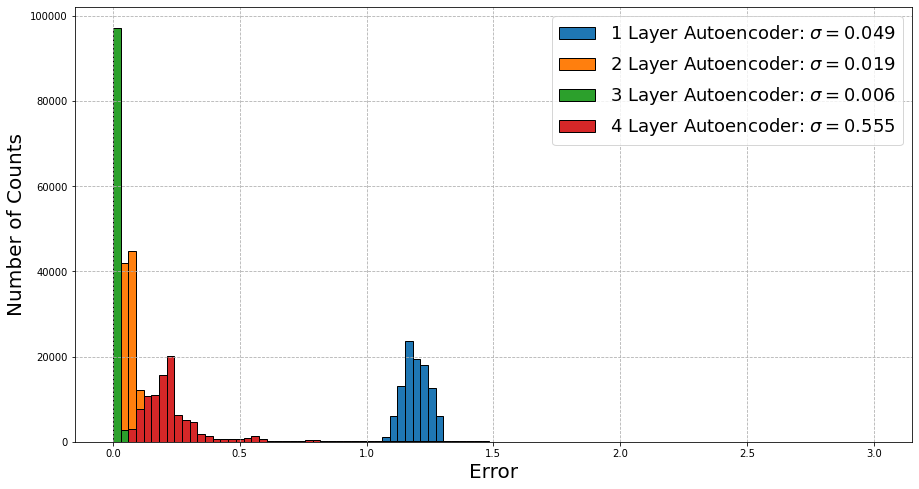
Wow now this is actually really interesting! We are actually seeing that this time around for correlated data, the performance increases if we increase the complexity of the autoencoder. At 3 layers, the accuracy and performance is extremely good, with the results being within 1% of the actual values. The performance seems to get worse past this point, which may point to the network trying to pick up on features that may not actually matter within this dataset (i.e., sometimes the data might start negative, which doesn’t really indicate anything important).

The MNIST Dataset

Okay enough messing around. As promised, we will now play with some actual data, and what better candidate than the “Hello World” dataset of machine learning - MNIST. The MNIST dataset is composed of hundreds of thousands of handwritten digits that are labeled with their corresponding digit. Let’s load in the data, normalize the pixel values to be between 0 and 1, and reshape the images from their standard 28x28 format to a more machine learning friendly 1x784.

(x_train, _), (x_test, _) = mnist.load_data()
x_train = (x_train.astype('float32') / 255.).reshape(len(x_train), len(x_train[0])*len(x_train[0][0]))
x_test = (x_test.astype('float32') / 255.).reshape(len(x_test), len(x_test[0])*len(x_test[0][0]))

For the model we will follow the same methodlogy as for the simple model from above, having one encoder layer and one decoder layer. The hidden layer in the model will contain 32 nodes, essentially performing a dimensionality reduction of 784/32 = 24.5. After running the model on the new training data, we can then look at some of the results:

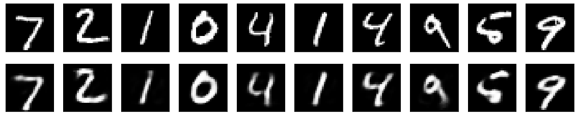
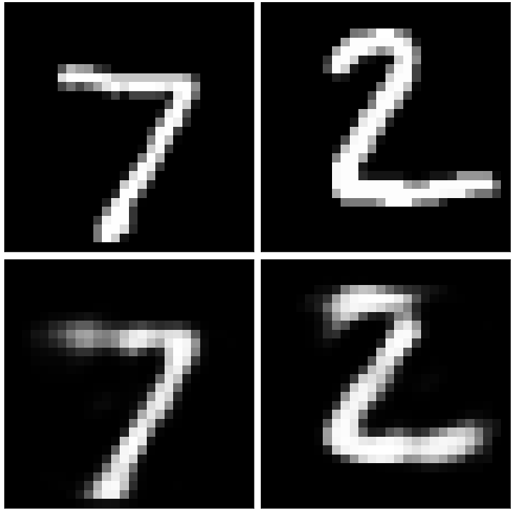
The original images can be seen on the top row, and the reconstructed images after being passed through the autoencoder can be seen on the bottom row. In general, the reconstructed images strongly resemble their originals, with the values of some of the pixels having been either enhanced or reduced. We can additionally select out some of the images with the worst performance:

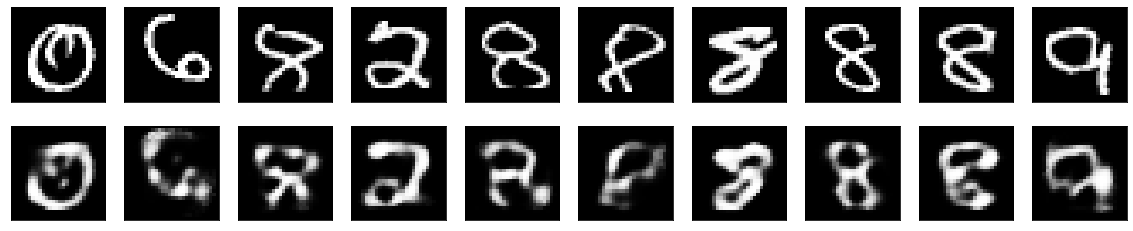
As well as some of the images with the best performance:

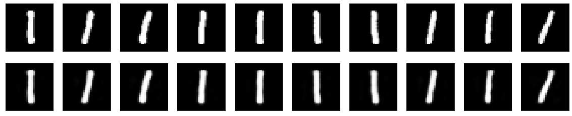
Interestingly enough, almost all of the images that contain a ‘1’ are the easiest for the model to reconstruct, presumably since this number is the simplest of the given digits, and doesn’t really contain any complex structure, such as loops or curves. It seems as though it has the hardest time with any number that contains a loop, such as ‘0,’ ‘6,’ ‘8,’ ‘9,’ and occasionally ‘2’ (depending on how it was written).